Motion: Attractor
- Author:
- Juan Carlos Ponce Campuzano
Now that we have implemented motion with velocity and acceleration, let’s try something a bit more complex and a great deal more useful. We’ll dynamically calculate a ball’s acceleration according to the following condition:
Acceleration towards a given point.
Anytime we want to calculate a vector based on a rule or a formula, we need to compute two things: magnitude and direction. Let’s start with direction. We know the acceleration vector should point from the ball’s location towards the point's location. Let’s say the ball is located at the point (x,y) and the point at (x', y').
In the following Figure we see that we can get a vector (dx,dy) by subtracting the ball’s location from the point’s location.
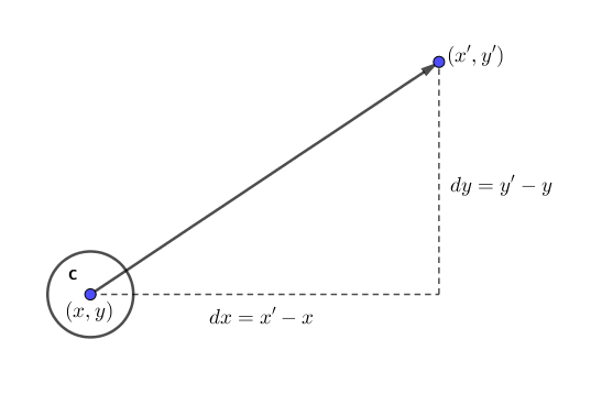
If the ball were to actually accelerate using that vector, it would appear instantaneously at the point's location. This does not make for good animation, of course, and what we want to do now is decide how quickly that ball should accelerate toward that given point.
In order to set the magnitude (whatever it may be) of our acceleration, we must first normalize that direction vector. That’s right, normalize. If we can shrink the vector down to its unit vector (of length one) then we have a vector that tells us the direction and can easily be scaled to any value.
To summarize, we take the following steps:
- Calculate a vector that points from the object to the target location (the given point)
- Normalize that vector (reducing its length to 1)
- Scale that vector to an appropriate value (by multiplying it by some value)
- Assign that vector to acceleration
Thus the script in the Setup button is:
##My circle or ball
xloc=5
yloc=5
SetValue(xloc, 5)
SetValue(yloc, 5)

O=(xloc, yloc)

c=Circle(O, 1)

##Velocity
xvel=Slider(-0.3, 0.3, 0.001, 1, 140, false, true, false, false)
yvel=Slider(-0.3, 0.3, 0.001, 1, 140, false, true, false, false)
SetValue(xvel, RandomUniform(-0.3, 0.3))
SetValue(yvel, RandomUniform(-0.3, 0.3))

##Attractor
Ax=Slider(-15,15, 0.001, 1, 140, false, true, false, false)
Ay=Slider(-10,10, 0.001, 1, 140, false, true, false, false)

A=(Ax, Ay)

#direction
dx=Ax-xloc
dy=Ay-yloc
norm=sqrt(dx^2+dy^2)
scale=0.06

#Normalize and scale
dxn=(Ax-xloc)/norm*scale
dyn=(Ay-yloc)/norm*scale

##Acceleration
xacc=dxn
yacc=dyn

Run=Slider(-5, 5, 0.01, 1, 140, false, true, false, false)

Box=Polygon((-15, -10), (15,-10), (15, 10), (-15, 10))
Finally, the slider Run should have the following script:
#Update velocity
SetValue(xvel, xvel + xacc)
SetValue(yvel, yvel + yacc)
#Update location
SetValue(xloc, xloc+xvel)
SetValue(yloc, yloc+yvel)
The following applet shows this implementation.Attractor implementation
You may be wondering why the circle doesn’t stop when it reaches the target. It’s important to note that the object moving has no knowledge about trying to stop at a destination; it only knows where the destination is and tries to go there as quickly as possible. Going as quickly as possible means it will inevitably overshoot the location and have to turn around, again going as quickly as possible towards the destination, overshooting it again, and so on and so forth.
This example is remarkably close to the concept of gravitational attraction (in which the object is attracted to the given point). However, one thing missing here is that the strength of gravity (magnitude of acceleration) is inversely proportional to distance. This means that the closer the object is to the attractor, the faster it accelerates.