Inside the Trefoil knot inside Torus
Instructions - Part I
Open GeoGebra in your desktop. Activate 2d and 3d graphics. You will be able to create a Torus with a trefoil knot inside. This is done using vector calculus, which requires lots of computations for the software, so you will need to have a powerful computer. The picture below shows an example of the result.

Instructions - Part II
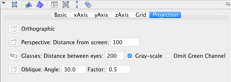
To have an interesting view in the 3d graphic, open the properties and go to the Projection tab. Choose Perspective option and type 100, as shown in the following picture:
Instructions - Part III
In the 2d graphics, create a button with the following GGB Script:
#First define the components of the trefoil knot Curve (it could be another curve in space R^3)
fx(x)=(2 + cos(3 / 2 x)) cos(x)-2
fy(x)=(2 + cos(3 / 2 x)) sin(x)
fz(x)=sin(3 / 2 x)
SetVisibleInView(fx,1,false)
SetVisibleInView(fy,1,false)
SetVisibleInView(fz,1,false)
SetVisibleInView(fx,-1,false)
SetVisibleInView(fy,-1,false)
SetVisibleInView(fz,-1,false)
#This defines the curve. To plot it write true below.
f=Curve(fx(t),fy(t),fz(t), t, 0, 4π)
SetVisibleInView(f,-1,false)
#Calculate derivative of each component of the curve
dfx(x)=Derivative(fx)
dfy(x)=Derivative(fy)
dfz(x)=Derivative(fz)
SetVisibleInView(dfx,1,false)
SetVisibleInView(dfy,1,false)
SetVisibleInView(dfz,1,false)
SetVisibleInView(dfx,-1,false)
SetVisibleInView(dfy,-1,false)
SetVisibleInView(dfz,-1,false)
v1=Curve(0,-dfx(t)/sqrt(dfx(t)*dfx(t)),0,t,0,4pi)
SetVisibleInView(v1,1,false)
SetVisibleInView(v1,-1,false)
v2=Curve(dfx(t)*dfz(t)/sqrt((dfx(t)*dfz(t))^2 + (dfx(t)*dfx(t))^2),0,-dfx(t)*dfx(t)/sqrt((dfx(t)*dfz(t))^2 + (dfx(t)*dfx(t))^2), t, 0, 4π)
SetVisibleInView(v2,1,false)
SetVisibleInView(v2,-1,false)
#Recall that "f=Curve(fx(t),fy(t),fz(t), t, 0, 4π)"
#Now we define the components of the parametric surface.
gx(x,y)=fx(x)+(cos(y)*0+sin(y)*(dfx(x)*dfz(x)/sqrt((dfx(x)*dfz(x))^2 + (dfx(x)*dfx(x))^2) ) )/2
gy(x,y)=fy(x)+(cos(y)*( -dfx(x)/sqrt(dfx(x)*dfx(x)) )+sin(y)*0)/2
gz(x,y)=fz(x)+(cos(y)*0+sin(y)*( -dfx(x)*dfx(x)/sqrt((dfx(x)*dfz(x))^2 + (dfx(x)*dfx(x))^2) ) )/2
SetVisibleInView(gx,1,false)
SetVisibleInView(gy,1,false)
SetVisibleInView(gz,1,false)
SetVisibleInView(gx,-1,false)
SetVisibleInView(gy,-1,false)
SetVisibleInView(gz,-1,false)
#Uncomment the next two lines, if you wan to plot
#knotS=Surface(gx(t,theta),gy(t,theta), gz(t,theta), t, 0, 4 pi, theta, 0, 2 pi)
#SetVisibleInView(knotS,-1,true)
#We will take a projection to S^3
#define by
#s3Proj=v/norm(v)^2
#for a particular value on the surface, which is defined by the function f.
value=2/3 pi
#We need to define the norm separately considering the point "f(value)"
normgf2(x,y)=(gx -fx(value))^2+(gy-fy(value))^2+(gz-fz(value))^2
SetVisibleInView(normgf2,-1,false)
#This is the result
torusKnot=Surface((gx(t,theta)-fx(value))/normgf2(t,theta),(gy(t,theta)-fy(value))/normgf2(t,theta), (gz(t,theta)-fz(value))/normgf2(t,theta), t, 0, 4 pi, theta, 0, 2 pi)
SetVisibleInView(torusKnot,-1,false)
#Finally, we just rotate a little to make it look cooler.
rotY=Slider(-pi,pi,pi/10,1,100,false,true,false,false)
SetValue(rotY,-pi/4)
torusKnotRotY=Rotate(torusKnot,rotY,yAxis)
SetVisibleInView(torusKnotRotY,-1,false)
rotX=Slider(-pi,pi,pi/10,1,100,false,true,false,false)
SetValue(rotX,0.27)
torusKnotRotX=Rotate(torusKnotRotY,rotX,xAxis)
Final comments
There might be a more efficient method to do all this in GeoGebra. If you find one, let me know: j.ponce@uq.edu.au
Another version that runs faster (online and in desktop) is here: Inside the Torus with a Trefoil knot