The Recursive Partitioning Supervised Machine Learning Algorithm

Author:: Greg Petrics

Topic:: Statistics

Introduction & Background

The supervised machine learning algorithm recursive partitioning (or "rpart" for short) is a classification algorithm that builds a decision tree model which can be used by a human being for classification. Because decision tree models are easily explainable and useable by humans, rpart is particularly useful for building tools for medical diagnoses in a clinical setting. Decision trees are also useful in any setting where data based decisions are required, but it is not practical to implement a statistical computation before the decision is made. The rpart algorithm is trained on data with any number of numerical or categorical explanatory variables, and a single categorical response variable with any number of levels. The algorithm works by recursively partitioning the explanatory variables into the "purest groups" of two of the levels of the response variable. The partition into the purest groups is accomplished by careful selection of a single splitting point in one of the explanatory variables. Assessment of the purity of the resulting groups is decided by any number of metrics, but the most commonly used metric is the gini index. This page will not get into the details of the gini index, and instead purity will be contemplated intuitively (see the interactive example below). It's most important to conceptually understand the first partition of an rpart model, because later partitions all adhere to the same principle. The first partition in an rpart model is the partition in one of the explanatory variables that simultaneously maximizes the (conditional) proportion of exactly two levels of the response variable on separate sides of the partition. This is sometimes informally described as partitioning the data into the "purest groups"; another informal description is to say that the partition has "maximized information" or induced "reverse entropy". See the interactive example below to help you understand this principle and these informal descriptions. After the first partition is determined by rpart, partitioning continues recursively (hence the name) on each of the resulting partitions until some stopping criteria is satisfied. Stopping criteria include having achieved a certain number of partitions, a certain limit on the size of a partition, or an inability to split partitions into purer groups. These criteria are all fairly technical and are not addressed in this tutorial. Once recursive partitioning has stopped, the resulting partitions can be interpreted as a decision tree. The highest proportion of a level of the explanatory variable in each final partition is used as the classification of that partition. Because the partitioning occurs in a binary fashion, there is a unique path from the entire data set to each partition by way of splits in the explanatory variables. As such, each partition path from the entire data set down to a final partition can be thought of as a branch in a decision tree. See further down in this this tutorial for an exmaple. Model performance of a rpart model is not usually assessed by p-values as in regression models. Instead rpart model skill is typically judged by the proportion of predictions the model gets correct on unseen "testing" data (i.e. data in which the classifications are known but the model was not trained on). Higher proportions of correct predictions are better, and are usually assessed against what might be expected if random classifications were made. It is also common to use confusion matrices. This page does not talk about model skill or confusion matrices. Check back later for a separate tutorial on those concepts.

An Interactive Example (The First Split)

The first two applets below help you explore the first partition of a recursive partitioning. In Applet 1 and Applet 2 the plotted colored dots represent a training data set with two numerical explanatory variables, and a single three-level categorical response variable. The training data is the same in both applets. The two explanatory variables range from about 20 to 80 in x, and 0 to 9 in y. The plane the dots are plotted in is the explanatory space, and in this example it is the 2 dimensional Euclidean plane. Additional explanatory variables increase the dimensions of the explanatory space. The single categorical response variable is plotted as the color of the dots. There are three levels of the response variable: level 1 is red, level 2 is green, and level 3 is Blue. In case you are curious, the data are the results of a survey of people's favorite Star Wars Trilogy in the Skywalker Saga. The horizontal axis is the respondent's age in years. The vertical axis is the number of Skywalker Saga films the respondent has seen (0 on up to all 9 films). The color of the dot represent's the respondent's self-reported favorite trilogy; level 1 is the Prequel Trilogy (Episodes 1-3, 1999-2005), level 2 is the Original Trilogy (Episodes 4-6, 1977-1984), and level 3 is the Sequel Trilogy (Episodes 7-9, 2015-2019). In this example, the rpart algorithm will attempt to use this training data to build a model to predict a person's favorite trilogy as a response to their age ("Age" or x-axis) and the number of Star Wars Movies they've seen ("Movies Seen" or y-axis). The gray points (and dependent segments) in the applets represent proposed first splits in the "Age" (Applet 1) and "Movies Seen" (Applet 2) explanatory variables. We need to pick one split in one of the explanatory variables. The recursive partitioning algorithm examines all possible splits of the data set in both explanatory variables, and seeks the point in one of them that simultaneously maximizes the conditional proportion of two different Trilogy Preferences on different sides of the partition. At the outset, in Applet 1, "Age" is split at about 10 years, and in Applet 2, "Movies Seen" is split at about 1 movie. These splits both result in poor purity in the resulting partitions. For instance, in Applet 1, the age of all respondents is older than 10 years, and so there is no data (and no proportion) on the left, and all data is on the right. The proportions are all maximized, but they are not simultaneously maximized on two sides of the partition. You can engage with these applets by adjusting the gray points to explore different splits in the "Age" and "Movies Seen" variables. As you adjust a gray point, the color of the partitions will change when one of the Trilogy preference conditional proportions in the partition exceeds all the others. At the outset, in Applet 1, there is no highest proportion on the left side of the partition (since every case of all three levels is on the right), and so the left is gray. The right partition is green however because the Original Trilogy is preferred on this side by 41 out of all 56 respondents who are older than 10 (which is all respondents). In Applet 2 however, both the bottom and top partitions are green because preference for the Original Trilogy dominates in both the top and bottom partitions. Adjust the splits. As you do so the counts of each preference and the size of each group in all partitions is automatically tabulated in the tables on the right. Try to find the split in either "Age" or "Movies Seen" that simultaneously maximizes two of the three preference proportions on both sides of the partition.

Applet 1 -- Exploring Splits in "Age"

Applet 2 -- Exploring Splits in "Movies Seen"

After exploring the splits in both "Age" and "Movies Seen" you should note that the purest split appears to occur by splitting "Age" (Applet 1) somewhere between 29 or 31; the gini index prioritizes proportions closer to 1, and so the split at 31 is considered optimal. With a split in "Age" at 31 observe that 36 of the 39 respondents in the right partition (92%) favor the Original Trilogy, and 8 of the 17 respondents in the left partition (47%) favor the Prequel Trilogy. No other split in "Age" or "Seen" results in a higher simultaneous pair of conditional proportions (In fact no partition in "Movies Seen" offers much purity in the groups). As such, the first partition of a recursive partitioning of this data set is at Age = 31.

Interactive Example Continued (The Second Split)

After the first split and resulting partitions are established, the rpart algorithm continues on each partition just as before. As described in the Introduction rpart will continue splitting partitions until a complexity criterion is met. In this particular training data additional purity can be achieved on the left with a split of "Movies Seen" at 1. See Applet 3 below which will help you see this for yourself. In Applet 3 the split in "Age" at 31 is now fixed, and you can explore splits in the left partition in "Movies Seen". The tables on the right have been updated to only reflect conditional proportions of the top and bottom in the left partition (respondents younger than 31). Try it out! Can you find a pure split?

Applet 3 (The Second Split in "Movies Seen")

After exploring in Applet 3, you should notice that an optimal split of the left partition (respondents younger than 31) occurs with "Movies Seen" at about 1. With a split in "Movies Seen" at 1 observe that 8 of the 12 respondents in the top partition (67%) favor the Prequel Trilogy, and 3 of the 5 respondents in the bottom partition (60%) favor the Sequel Trilogy. This agrees with an observation by some Star Wars fans that the only people who like the Sequel Trilogy are those who are young and haven't seen many of the Star Wars movies. Note: I have not provided additional applets to explore splits in "Age" in the left partition or "Age" or "Movies Seen" in the right partition. It is a fact that very little increase in purity is possible by exploring splits in these explanatory variables. Partitioning could continue beyond this second split (in particular the top partition), but this is a good place to stop since the purpose of this tutorial was only to help you understand the theory behind the algorithm.

Decision Trees (Summaries of RPart Models)

The recursive partitioning we've explored above is nicely summarized in a decision tree. See below. Note: A description of decision trees can be found above in the Introduction & Background.

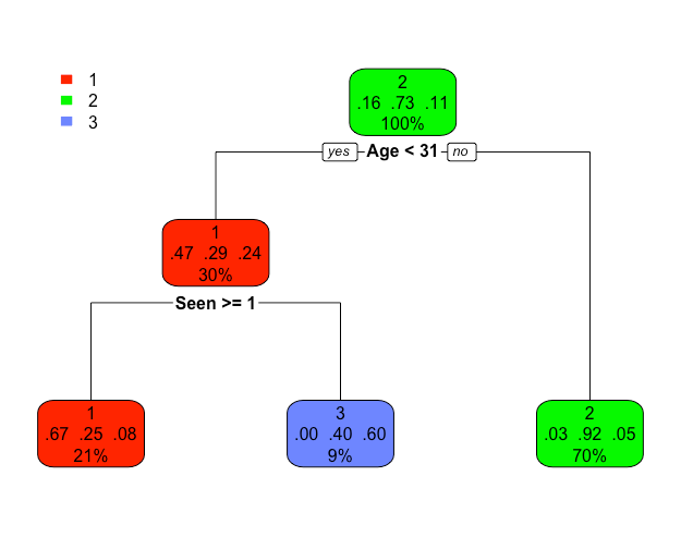
Each path from the top to the bottom of the decision tree represents a "data based decision" about a person's favorite Trilogy in response to their age and the number of Star Wars movies they've seen (0 to 9). For instance the left path can be read: "if a person is less than 31 years old and seen 1 or more movie, then the model predicts they will prefer Trilogy 1 (the Prequel Trilogy)". The right most path can be read: "if a person is 31 years or older; the model predicts they will prefer Trilogy 2 (the Original Trilogy)". Note that no information about the number of movies seen is needed to make the decision represented by the right leaf. The proportions in each node are the conditional proportions of each level of the response variable in the node. We have encountered some of these proportions in our exploration of Applets 1, 2 and 3 above. Note that these proportions are sometimes interpreted as a probability of each possible classification decision. So for instance, in the lower left node, the proportion 0.67 indicates that in this node (younger than 31 and seen 1 or more movie) 67% of the participants prefer the Prequel Trilogy and furthermore, it can be interpreted as saying that there is a 67% probability a person in this node will prefer the Prequel trilogy. This was the same proportion / percentage that we discovered when interacting with Applet 3 above and finding the second split in "Movies Seen". The percentages in the bottom of each node represent the percent of the entire data set each node represents. So, for instance, the 21% in the lower left node indicates that 21% of respondents are younger than 31 and have seen 1 or more Star Wars movie. Note that the percentages across the bottom of the decision tree sum to 100% since all of the data eventually makes its way into some decision / partition.

Discussion questions:

1. Why do you think the model did not need any additional information about the number of movies seen for the lower right node? 2. Can you explain the decision represented by the middle leaf in plain English? 3. Can you explain in plain English what the meaning of 0.80 is in the middle leaf?