Optimization Application - 3D Model

Author:: rabani_dhillon

Background

Throughout our studies of calculus, we have examined several knowledge-based applications of derivatives. Oftentimes students underestimate the practicality behind these concepts and whether or not this learning can be applied in the real world. In this lesson, we will dive headfirst into the world of calculus by solving an engaging optimization problem that involves a real-life application of derivatives. Although optimization has been covered in the curriculum of this course, this particular application enables us to go beyond and expand on our prior understanding through the incorporation of a more complex shape in 3D and a total cost relative to each dimension. The foundational concepts of calculus are involved through the differentiation of a cost function, using the first derivative to find critical numbers, and an application of the second derivative test to classify local extremes. So let's get started!

Optimization Problem

The vaccine for COVID-19 was recently discovered and will be packaged into cylindrical vials with a volume of 350cm³. Find the dimensions that will minimize the surface area of the vial. If the aluminum used for the lid costs $0.50/cm², and the glass for the sides and bottom costs $0.30/cm², what is the minimum cost that the manufacturing plant must pay to produce the container of each vaccine? Round all answers to 2 decimal places.

(Animation) What dimensions will optimize its surface area and cost?

3D Model Corresponding to Properties of the Vial

Solution

Throughout the process of problem-solving, you may interact with the model to visualize the shape of the vial.

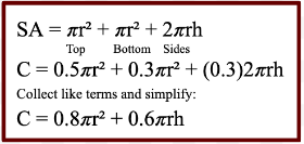
Step 1: We are interested in finding a value of the cylinder's radius and height that minimizes the surface area, thereby minimizing the cost of each vial. You might recognize the constraint is that the volume must be equal to 350cm³. This is simply a given requirement that must be fulfilled by the unknown dimensions of the vial. Firstly, we would use the known properties to create a cost equation. Refer to the steps below to do so. After forming this equation, you will notice that there are two variables in the cost equation (r and h). However, this inhibits us from using algebra to isolate and solve for a variable. We need to subsequently formulate a cost function that is written in terms of one variable.

Begin by defining each variable; Let C = the total cost, let
r = the vial's radius, and let h = the vial's height. We need to input
the cost relative to each dimension into the surface area
formula of a cylinder. Recall that the lid on top costs $0.50/cm²,
and glass on the sides and bottom cost $0.30/cm². Simplify
further by collecting like terms. — Begin by defining each variable; Let C = the total cost, let r = the vial's radius, and let h = the vial's height. We need to input the cost relative to each dimension into the surface area formula of a cylinder. Recall that the lid on top costs $0.50/cm², and glass on the sides and bottom cost $0.30/cm². Simplify further by collecting like terms.

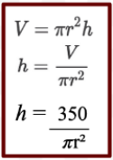
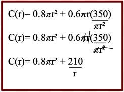
Step 2: In the animation of this model, recall that the value of the volume remained constant regardless of the possible dimensions of the vial. We will now rearrange the equation of the constraint to isolate a variable. Refer to the steps below. Afterward we will replace this equivalent equation into the cost equation to create a function for the cost of each vial. See the detailed process below.

In this case, we will need to rearrange to
formula of the volume to isolate for h by
dividing the V by πr². From here we simply
input the value of the volume which is 350cm³
in for V. — In this case, we will need to rearrange to formula of the volume to isolate for h by dividing the V by πr². From here we simply input the value of the volume which is 350cm³ in for V.

We can sub this into the cost equation for h.
Cancel out the factors (πr) to simplify. This is
our cost function. — We can sub this into the cost equation for h. Cancel out the factors (πr) to simplify. This is our cost function.

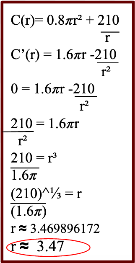
Step 3: To find our local extreme values we must differentiate the cost function and use the first derivative to find critical numbers. Refer to the specific steps of this process below.

Apply the power rule on the first term and the quotient
rule on the second term to find the first derivative. To
find the critical numbers we will set C’(r)=0 where r>0.
Next, we need to rearrange the setup to isolate for r
using algebra. Move the second term to the left side,
move 1.6π along into the denominator, and move the r²
onto the right side. Proceed to cube root the term to
evaluate for r which is approximately equal to 3.47cm. — Apply the power rule on the first term and the quotient rule on the second term to find the first derivative. To find the critical numbers we will set C’(r)=0 where r>0. Next, we need to rearrange the setup to isolate for r using algebra. Move the second term to the left side, move 1.6π along into the denominator, and move the r² onto the right side. Proceed to cube root the term to evaluate for r which is approximately equal to 3.47cm.

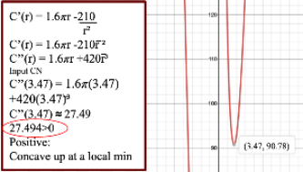
Step 4: Next, we will use the second derivative to test for concavity and classify our critical number as a local max or min. To do so, we need to differentiate the first derivative and plug our critical number into the equation of the second derivative. For visual learners, the graph of the cost function can be found below. This may be used to verify our classification of this point as it is evidently a local minimum.

Apply to the power rule on both terms to find the second derivative.
Then proceed to sub in the critical number, 3.47 into the equation.
After calculating we get an answer of about 27.49 (a positive number).
Based on prior knowledge, we know the function will be concaving
up at this minimum point. It is conclusive that this value of the radius
minimizes the surface area and cost. — Apply to the power rule on both terms to find the second derivative. Then proceed to sub in the critical number, 3.47 into the equation. After calculating we get an answer of about 27.49 (a positive number). Based on prior knowledge, we know the function will be concaving up at this minimum point. It is conclusive that this value of the radius minimizes the surface area and cost.

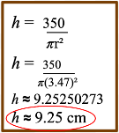
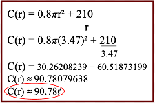
Step 5: Now that we have found the value of the radius that optimizes the surface area and cost of the cylinder, we need to find the corresponding dimension of the height and the total cost to produce each vial (the y value of this point). Refer to the steps of this process below.

Use the rearranged formula of the constraint
(from step 2) and sub in 3.47 for r to evaluate
its height. Upon calculating this, we reach an
answer of approximately 9.25cm for the
height of the vial. — Use the rearranged formula of the constraint (from step 2) and sub in 3.47 for r to evaluate its height. Upon calculating this, we reach an answer of approximately 9.25cm for the height of the vial.

Our final step is to input the value of the radius, 3.47 into
the original cost function for r and calculate it. The total cost
per vial is about 90.78¢. Recall that this is the same found
earlier (in step 4) through graphing the cost function. — Our final step is to input the value of the radius, 3.47 into the original cost function for r and calculate it. The total cost per vial is about 90.78¢. Recall that this is the same found earlier (in step 4) through graphing the cost function.

Conclusion

Altogether, we have verified our solution by interacting with the model and using graphing technology. For a clear overview of the model of the vial, refer to the diagram below which showcases the finalized dimensions of the vial in which the surface area and cost are minimized. We now need to conclude by providing a final sentence answer to the question: Therefore the dimensions that minimize the surface area of the vial are a radius of approximately 3.47cm and a height of approximately 9.25cm. The manufacturers will have to pay a minimum cost of approximately 90.78¢ to produce each vial in which the vaccines will be contained.

References

Optimization Problems. Sfu.ca. (2020). Retrieved 5 December 2020, from https://www.sfu.ca/math-coursenotes/Math%20157%20Course%20Notes /sec_Optimizati on.html Section 4-8 : Optimization. (2018). Retrieved 5 December 2020, from https://tutorial.math.lamar.edu/classes/calci/optimization.aspx