Branches of an implicitly defined biquadratic curve found using complex functions: Trifolium curve
Solving an implicitly defined plane curve means splitting it into separate "curve sections" for which explicit expressions of functional dependencies can be written. These may take the form of analytical function definitions, y = f(x), or parametrically defined curves where the x-coordinate coincides with the parameter, x = t.
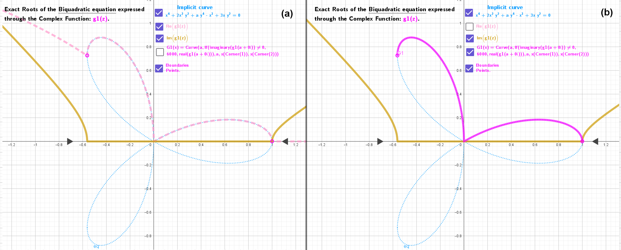
The applet considers the case of the Trifolium curve where an implicit equation of a plane curve is given in the form of a biquadratic equation in the variable y. Using its root formulas, 4 explicit functional dependencies of the real variable x are found that make up the plane curve under consideration. However, this method is not always applicable.
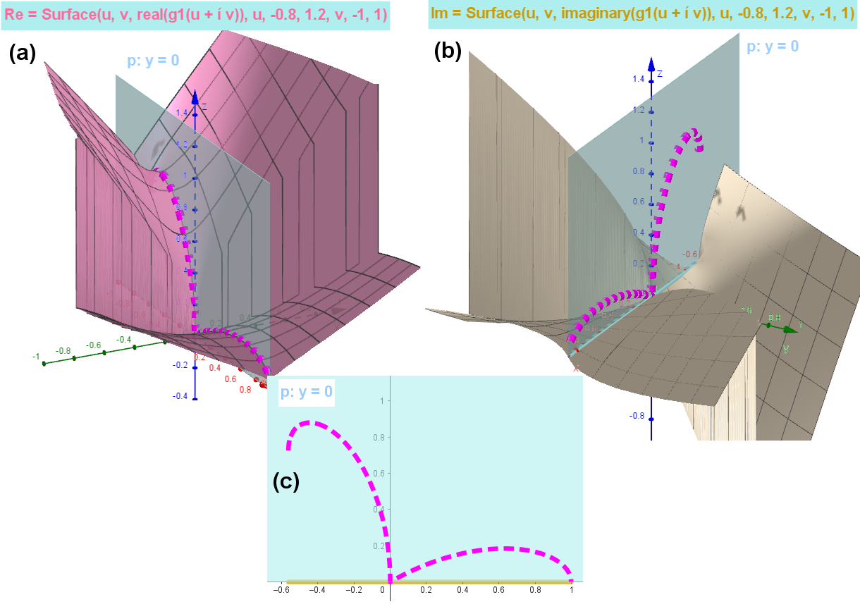
This applet illustrates the use of the method of parametrically defined complex functions to solve the same implicit biquadratic equation in y: eq: x⁴ + 2x² y² + a y⁴ - x³ + 3x y² = 0 . In the complex plane the variable x→z, y→f(z). The root formulas used are easily extended to the complex plane in a certain way. Roots: complex functions g1(z), g2(z), g3(z) and g4(z) are solutions of the corresponding complex equation.
Each of these functions f(z) has surfaces with real and imaginary parts (Fig. 1). In the problems considered, however, their values are only in the plane y=0 along the real x-Axis on the interval [a1,a2], where the imaginary part is zero. Curve(a,real(f(z)),a,a1,a2), where Curve(a,imaginary(f(z)),a1,a2)=0, is the part of the original plane curve on this interval. See the images Fig. 2 below the applet.
*Previous applet: Finding explicit expressions of four real functions for an implicitly defined plane curve whose equation is biquadratic in the variable y.